Financial news often attempt prediction of major index movements in terms of 'bad', 'gloomy' or 'rally' days for the markets based on the observed opening values. Here we would like to answer the question whether such a prediction is possible. To find the answer we study the Dow Jones industrial average values from 2003. The data show that a prediction is feasible, though the opening data are not enough. Historical data going at least three days back are necessary for a reasonable forecast.

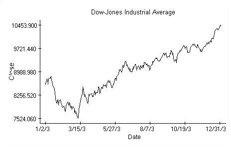
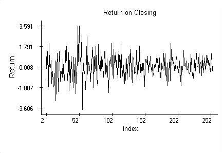
The intention is to provide evidence of dependence of the current closing value on the previous openings and closings using a linear regression theory argument. First we transform the original data, shown above, into observations from the Normal distribution by investigating the daily return, calculated according to the familiar formula

	rc[n]=100(c[n]-c[n-1])/c[n-1], 
		

where c[n] is the closing on day n. Similarly we calculate the return on opening and denote it

	ro[n]=100(o[n]-o[n-1])/o[n-1], 
		

where o[n] is the index value on New York market opening. The return values rc, computed from closings, are shown in the picture.

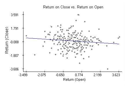
The regression of the return on closing against the return on opening is inconclusive and shows no relation between the opening and closing values. The regression coefficients become significant though once we include return on closing from the previous day. The diagnostic plots discussed next regard thus the model

	rc[n]=b[0]+b[1]ro[n]+b[2]rc[n-1]+e[n],
		

where b[0], b[1] and b[2] are estimated using the least squares method and e[n] are residuals of the model. Since the t-tests on coefficients b[1] and b[2] are significant on the 5% level, we have evidence of dependence of rc[n] on ro[n] and rc[n-1]. The coefficients b[1] and b[2] are recognized as significant also by the familiar Fisher's F-ratio testing the null hypothesis H0: b[1]=b[2]=0 vs. the hypothesis that at least one of the equalities fails. This points to dependence of c[n] on o[n], c[n-1], o[n-1] and c[n-2], because all these values must be known to get the necessary returns.

Regression analysis utilizes several basic data visualizations. First of all, plots of the dependent variable against the explanatory ones (partial plots). E.g. plot of the return on closing values against the returns on opening indicates a possible negative correlation emphasized by the regression line estimated by the least-squares method.

Regression analysis assumes the residuals of the model are independent,identically distributed Normal random variables. These assumptions areverified by plotting the residuals against the lag, against the predictions and calculations the autocorrelation and quantile plots. The plots are provided next and overall they support the assumptions except one.

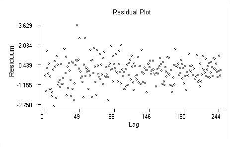
The plain residual plot indicates the variability of the returns may be changing (decreasing) over time. As the Dow-Jones average values peak, the daily returns decline. Time-dependent variability of market data is commonly recognized and must be handled using special classes of models.

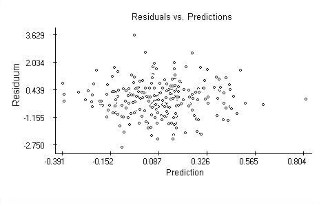
The residuals plotted against the predicted values are randomly scattered.

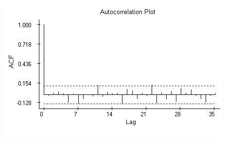
The autocorrelations appear not significant.

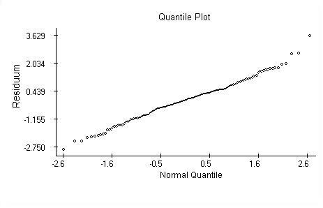
The quantile plot supports the Normal distribution hypothesis. The Kolmogorov-Smirnov test of normality also does not reject the null hypothesis.

To assure that the significance of the regression coefficients is not caused by some exceptional values, seven closing values (3% from the sample total) with highest Cook's distance have been dropped and the tests were re-evaluated. As to significance, the results have not changed. Though the model looks healthy up to the unsteady variance problem, for periods of data longer than one year the changing variance depreciates the fit up to a stage when the model is of no use. For the goal of this brief study the result is satisfactory.

Notes

A serious use of the above model for index return prediction requires answering of many questions. Here are some of them. Why estimate the model coefficients using exactly one year of data? Would it be better to use the most recent data rather than data from the previous year? Will inclusion of further returns from the past improve the prediction? Shall the structure of the model persist as new data arrive? Once we answer questions about the model, we will likely try to build strategies using the model to make profit or, more realistically, to reduce our investment risk. This is the part where computer modeling is very useful. A thorough introduction to linear regression analysis is

Draper, N. and Smith, H.: Applied Regression Analysis, Second Ed., Wiley, New York, 1981.

The data used in the example are available from the Yahoo finance web site.

Keywords

Linear regression, t-test, F-test, Cook's distance, Normal distribution, quantile plot, time series, residuals, modeling, prediction.